Knowing how to insert a check mark in Excel is a valuable skill to have, especially if you want to add a more professional, organized, and clean-cut look to your spreadsheets. Accessing check marks in Excel isn’t intuitive as it should be, but we’re here to help.
Fortunately, there are several ways that you can make check marks on Excel. You can use shortcuts or, if you prefer, navigate to a symbols dialog box manually and make Excel check marks that way. Without further ado, let’s check out how to make check marks in Excel.
How to insert a check mark in Excel (shortcut)
As mentioned, one way you can insert a check mark in Excel is to use a shortcut.
1. Place the cursor in the cell where you’d like to insert a check mark.
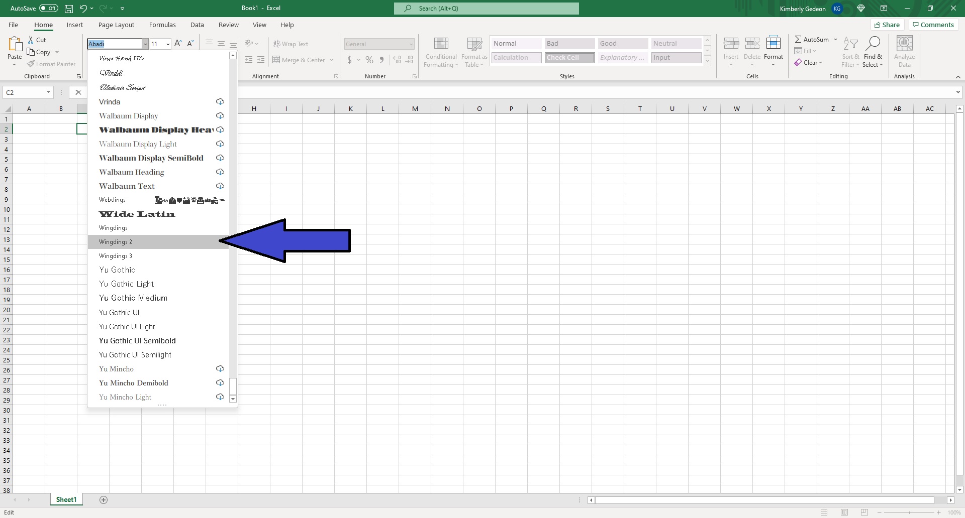
2. Change the font to Wingdings 2. And yes, it is must be Wingdings 2. I don’t know why there are several variants of this weird font, but I digress.
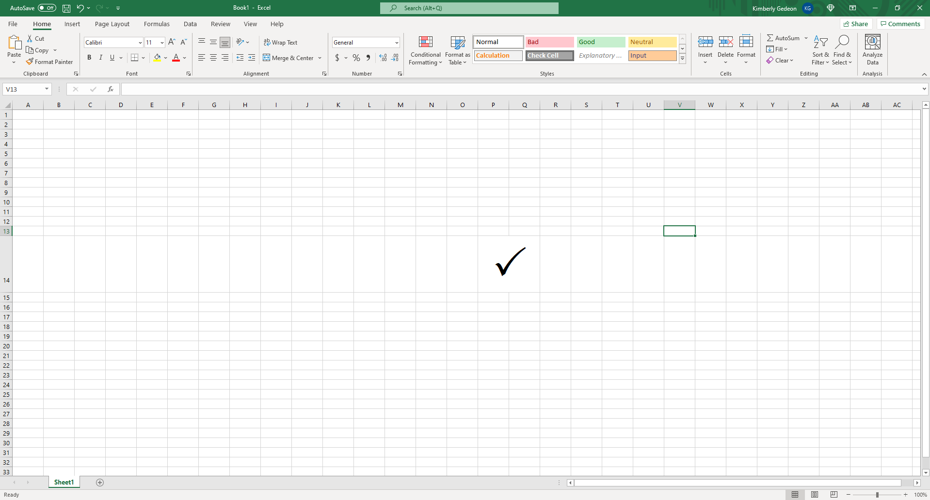
3. Press “ALT+P”. A check mark should appear.
How to insert a check mark in Excel (dialog box)
1. Click on the cell that you’d like to insert the check mark into.
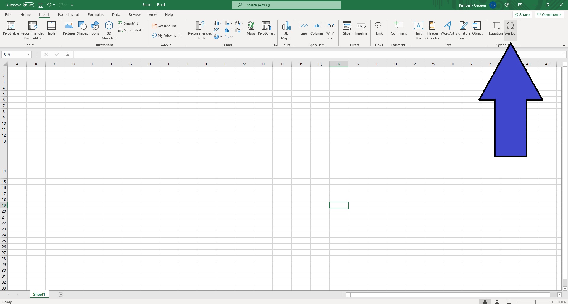
2. Open the “Insert” tab and click on “Symbol.”
2. When the Symbol dialog box pops up, type in “Wingdings 2” into the “font” field
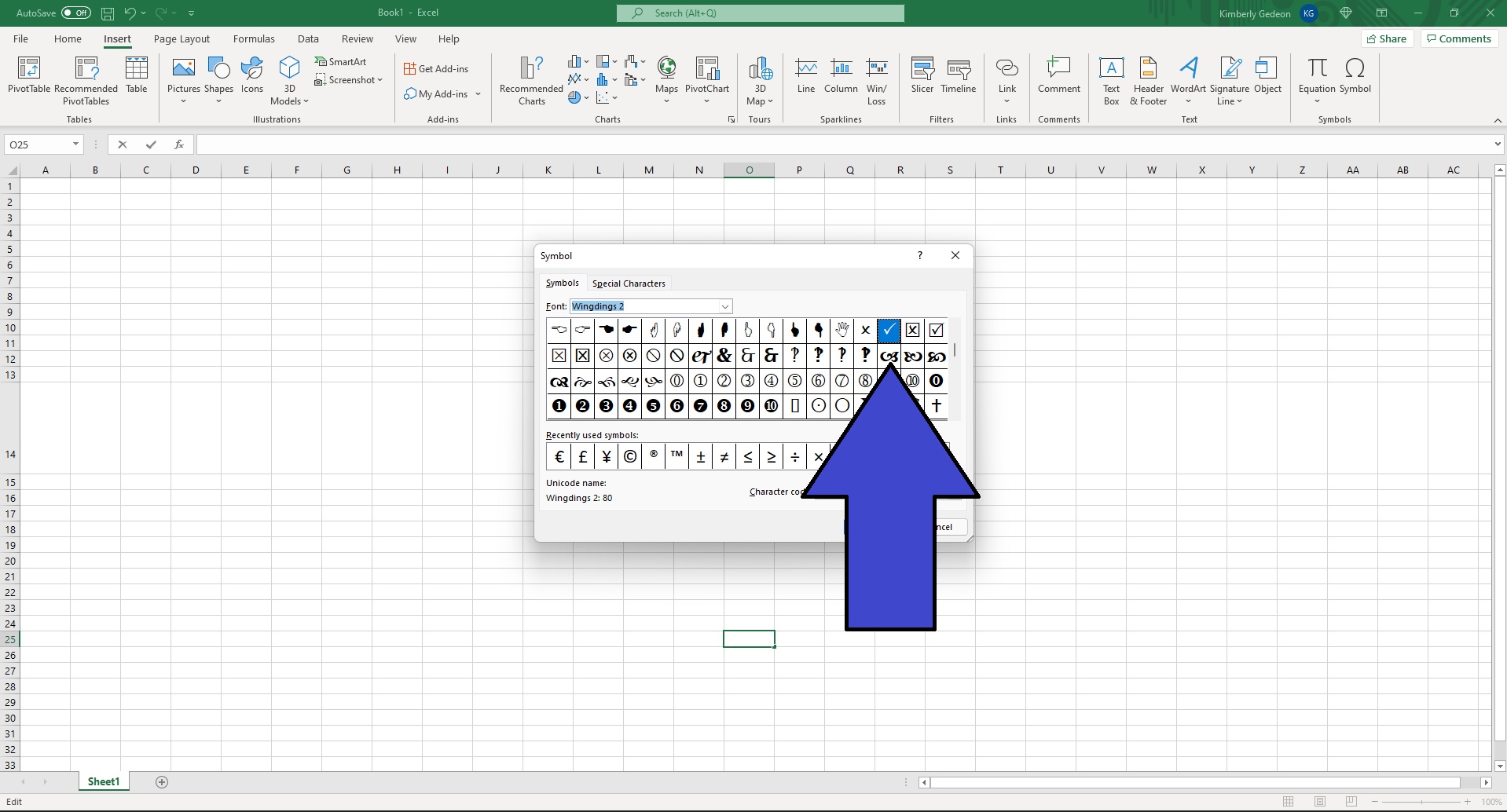
3. You’ll find two check mark symbols that you can use on Excel.
4. Click the one you prefer and click on “Insert.”
How to insert a check mark in Excel (Unichar function)
Perhaps the easiest way to insert a check mark in Excel is to use the UNICHAR function, a formula that translates numeric codes into corresponding characters. There are four UNICHAR codes that can manifest check marks in Excel: 9745, 9989, 10003, and 10004. Here’s how to get started.
1. Choose a cell where you’d like to insert your check mark.
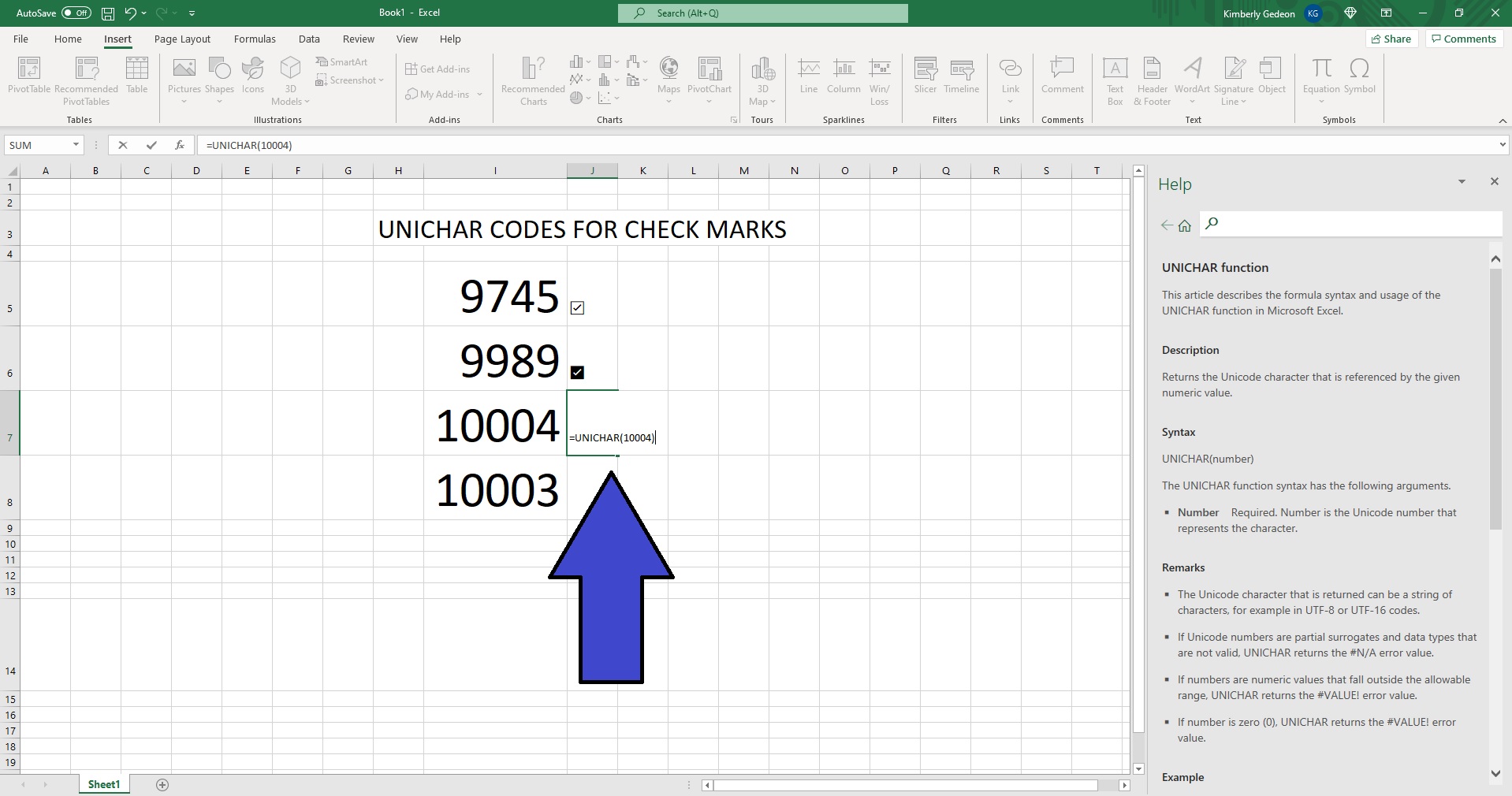
2. Type in “=UNICHAR” followed by one of the aforementioned codes wrapped in parentheses. For example, if you want to use the 10003 code, your input should look like the following: =UNICHAR(10003)
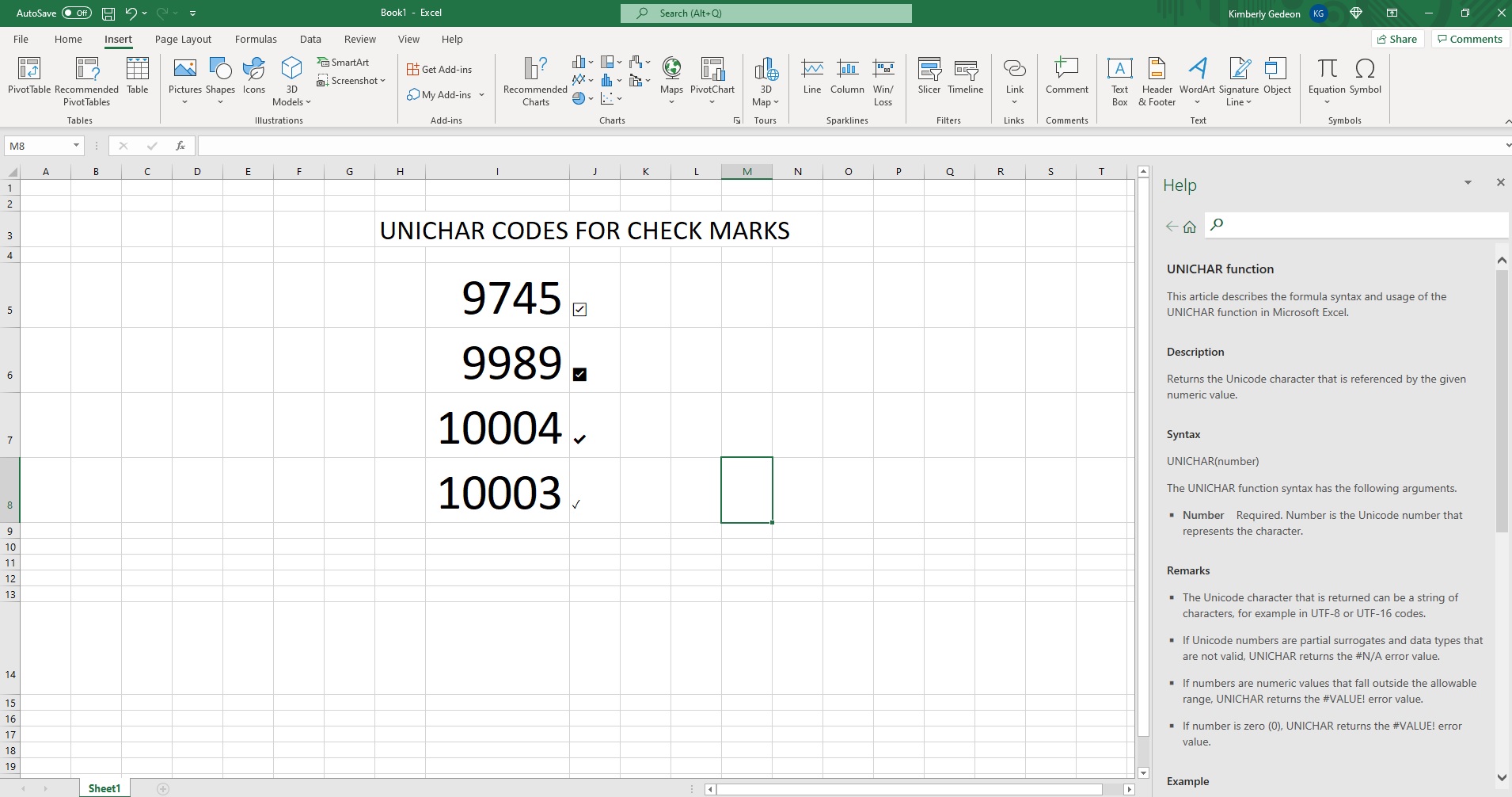
3. Hit “Enter” and the check mark should appear.